1. The problem
I have started the Coursera Machine Learning MOOC by Andrew Ng, see Coursera Machine Learning. In Coursera MOOC, all videos are downloadable from a main page where they are tagged with a duration in minutes, see for instance Machine Learning Video Lectures. I wondered if it was possible to predict the size in bytes of videos according to their tagged duration, for instance the first video Welcome (7 min) corresponds to a mp4 file of 12.531.478 bytes.
2. Getting tagged durations and video sizes automatically with Python
From the download page, we can see that each video is downloadable with the URL: https://class.coursera.org/ml-005/lecture/download.mp4?lecture_id=%i where the parameter is a video id (here, an integer between 1 and 114). Using Python, we can implement a function that gets the meta information for each video (without having to download it) and to extract the necessary information, i.e. the tagged durations (which are fortunately set in video filenames) as well as the video sizes in bytes.
The Python urllib2 library has all the necessary features to get these information automatically and a regular expression performs the extraction of the durations.
        import re
        import urllib2
        rx = re.compile("%20%28(\d+)%20min%29") # looking for ' (X min)' in video name
        course = 'ml-005' # course name
        fo = open("%s.txt" % course, "a")
        nvideos = 114
        for i in range(nvideos): # videos are numbered from 1 to nvideos
            try:
                u = urllib2.urlopen('https://class.coursera.org/%s/lecture/download.mp4?lecture_id=%i' % (course, i + 1))
            except: # in case a video is lacking
                continue
            meta = u.info() # meta-information of the page
            length = int(meta.getheaders("Content-Length")[0]) # length
            disposition = meta.getheaders("Content-Disposition")[0] # include filename
            m = rx.search(disposition) # looking for minutes
            if m:
                minutes = int(m.group(1))
            else:
                minutes = 0
            fo.write("%i\t%i\n" % (minutes, length))
            print i+1, minutes, length # display how the process is running
        fo.close()
This script generates a tabulated file named ml-005.txt with duration in minutes and size in bytes for each video, see the output file. In this MOOC, we can see that we get only 113 results since the video with id 94 is not referenced anymore.
3. Using linear regression to fit the data with Octave
Then, from the first programming exercice of the MOOC, using Octave to implement a linear regression with the gradient descent method on these data is quite straightforward.
        % GNUPLOT setting
        graphics_toolkit gnuplot

        %% Initialization
        clear ; close all; clc

        %% ======================= Part 1: Plotting =======================
        fprintf('Plotting Data ...\n')
        data = load('ml.txt');
        X = data(:, 1); y = data(:, 2)/1024/1024; % convert to MB
        m = length(y); % number of training examples

        plot(X, y, 'rx', 'MarkerSize', 10); % Plot the data
        ylabel('Size in MB'); % Set the y axis label
        xlabel('Duration in min'); % Set the x axis label

        %% =================== Part 2: Gradient descent ===================
        fprintf('Running Gradient Descent ...\n')

        X = [ones(m, 1), data(:,1)]; % Add a column of ones to x
        theta = zeros(2, 1); % initialize fitting parameters

        % Some gradient descent settings
        iterations = 1500;
        alpha = 0.01;

        % compute and display initial cost
        computeCost(X, y, theta)

        % run gradient descent
        theta = gradientDescent(X, y, theta, alpha, iterations);

        % print theta to screen
        fprintf('Theta found by gradient descent: ');
        fprintf('%f %f \n', theta(1), theta(2));

        %% ======================= Part 3: Plotting again =================
        % Plot Data
        hold on; % keep previous plot visible
        % Plot the linear fit
        plot(X(:,2), X*theta, '-')
        legend('Training data', 'Linear regression')
        hold off % don't overlay any more plots on this figure
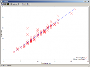
The octave script outputs finally a cost of 0.54824 and a theta vector of [0.407491 1.120686]. Therefore, the linear estimation of the video size in MB according to its tagged duration is given by the equation: y = θ0 + θ1.x
4. Graphical representation
The linear regression result is also displayed using Octave graphical features.
We can see that the data fit roughly to a straight line. In fact, the relationship between tagged durations and sizes is not linear since all videos may have not the same compression rate and the tagged durations may contain approximations or errors as well.
5. Compressing data with PCA in Octave
PCA script from Coursera can easily be adapted to compress these data. The top eigen vector is on the first bissector y = x.
        % GNUPLOT setting
        graphics_toolkit gnuplot

        %% Initialization
        clear ; close all; clc

        %  The following command loads the dataset. You should now have the
        %  variable X in your environment
        X = load('ml.txt');
        X(:, 2) = X(:, 2) / 1024 / 1024; % convert to MB

        %  Visualize the example dataset
        plot(X(:, 1), X(:, 2), 'bo');
        axis([0 25 0 25]); axis square;

        %  Before running PCA, it is important to first normalize X
        [X_norm, mu, sigma] = featureNormalize(X);

        %  Run PCA
        [U, S] = pca(X_norm);

        %  Compute mu, the mean of the each feature

        %  Plot the normalized dataset (returned from pca)
        plot(X_norm(:, 1), X_norm(:, 2), 'bo');
        axis([-4 4 -4 4]); axis square

        %  Project the data onto K = 1 dimension
        K = 1;
        Z = projectData(X_norm, U, K);

        X_rec  = recoverData(Z, U, K);

        %  Draw lines connecting the projected points to the original points
        hold on;
        plot(X_rec(:, 1), X_rec(:, 2), 'ro');
        for i = 1:size(X_norm, 1)
            drawLine(X_norm(i,:), X_rec(i,:), '--k', 'LineWidth', 1);
        end
        legend('Training data', 'PCA', "location", "southeast")
        hold off
Then the raw and the reconstructed data can be displayed on the same graph. Graphical comparison between linear regression (ordinary least squares) is explained in this post: Principal Component Analysis vs Ordinary Least Squares: a Visual Explanation. Examples are given in the R language.
6. To do…
Handling durations in the format MM:SS and managing problems in retrieving video meta-information.


Be the first to post a comment.